Tutorial 5. Compare trees derived from different genes

Summary:

This tutorial describes the use of RASP to compare trees derived from different genes of Ebolavirus as in Kendall and Caroline (2016). It will take you through the process of comparing trees, which extracts distinct alternative evolutionary relationships embedded in the data.

Information of data source

The sequence data from the Ebola virus samples, both historical and from the 2014 outbreak, were obtained from Gire et al. (2014). We selected 20 taxa and built trees following the method in Kendall and Caroline (2016). GP, L, NP, VP24, VP30, VP35 and VP40 are genes in the Ebola genome and "All" is all genes together. We sampled 100 trees from the posterior for each gene and "All", which are stored in examples/Ebola/Trees.

If you are a beginner of RASP, please start from Tutorial 1.

Loading the data files

Click [File> Close Current Data] or reopen RASP to clear the current trees.

Open [File > Load Trees> Load Trees (more format)] and navigate to Trees_States folder and select all of the .trees files. Each file contains 100 trees, which will result in 800 trees in total.

Calculate and visualize matrix of tree distances

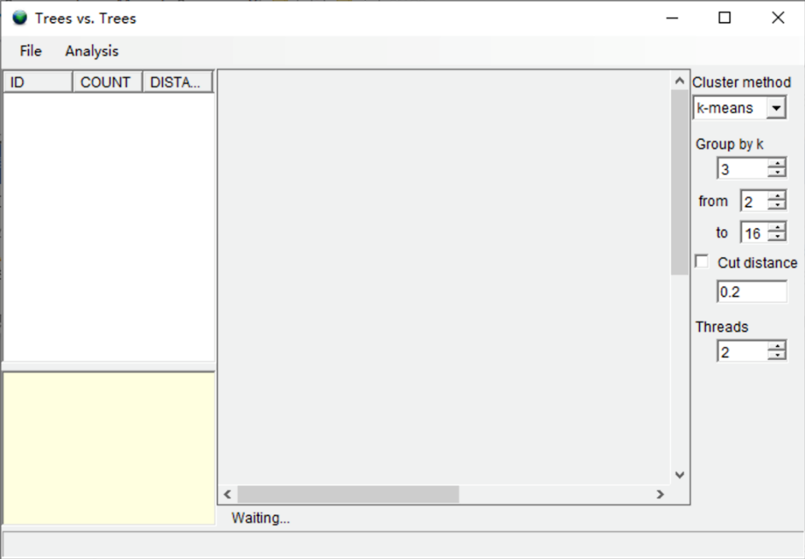
Open [Comparison> Trees vs. Tress], and you will see a window like this:

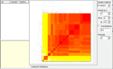
First, we comput pairwise distances between all these trees. Open [Analysis> Calculate Matrix> KC Distance]. You may see a command window (in Windows) with some additional information. Keep it open until it closes automatically. This analysis took about 5 second on a 3.0 GHz CPU). Open [Analysis> Heatmap> Make Heatmap] to visualize tree distances, and you will see a window like this:

Test the number of clusters and cluster trees

Open [Analysis> Cluster Trees> Test k]. You can keep everything as default and click “Run”. Users may see a command window (in Windows) with some additional information. Keep it open until it closes automatically. The analysis took about 30 second on a 3.0 GHz CPU). You can use the k value detected by RASP (Gray line) to set the value of “Group of k”. Then you will see a window like this:

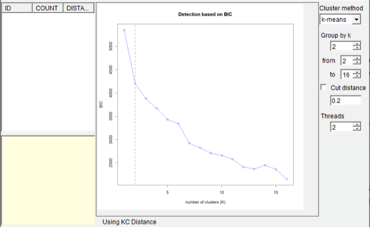
NOTE. If you are using k-means method, RASP chooses the number of clusters according to the Bayesian Information Criterion (BIC). If you are using other methods, RASP will not choose the number of clusters automatically. You should choose the number of clusters according to the graphic of k.

Select [Analysis> Cluster Trees> Hierarchical Cluster]. You may see a command window (in Windows) with some additional information. Keep it open until it closes automatically. This analysis took about 30 second on a 3.0 GHz CPU. When finished, you will see a window like this:

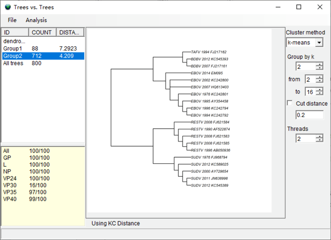
Select the group with largest number of trees (COUNT column). In our result, we select Group2. The summary of trees in the bottom left shows that the trees generated from VP30 do not cluster with other genes (16 of 100), which indicates that the VP30 gene has a distinct phylogenetic signature. The right window shows the consensus tree of the selected group. Users should carefully examine the consensus trees of the two groups and “All trees,” as the topology of each tree may differ substantially.

NOTE: Changing the clustering method (e.g. ward.D, ward.D2, single, etc.) will change the clustering of the trees slightly. However, if you change the method of calculating the matrix of tree distances, the result may change substantially. See discussion in Kendall and Caroline (2016) for more information.

Inferring ancestral states from the distinct clusters

In this part, we use simulated state data to reconstruct ancestral states from distinct clusters.

Open [File> Save> Save ALL] to save all trees and data. Back on the main window, click [File> Close Current Data] or reopen RASP to clear the current trees. In this tutorial, we saved the files in the Results folder.

Open [File > Load Trees> Load Trees (more format)] and navigate to Results/group1.trees and select it.

Open [File> Load Consensus Tree> Load User-specified Tree] and navigate to Results/group1_con.tre and select it.

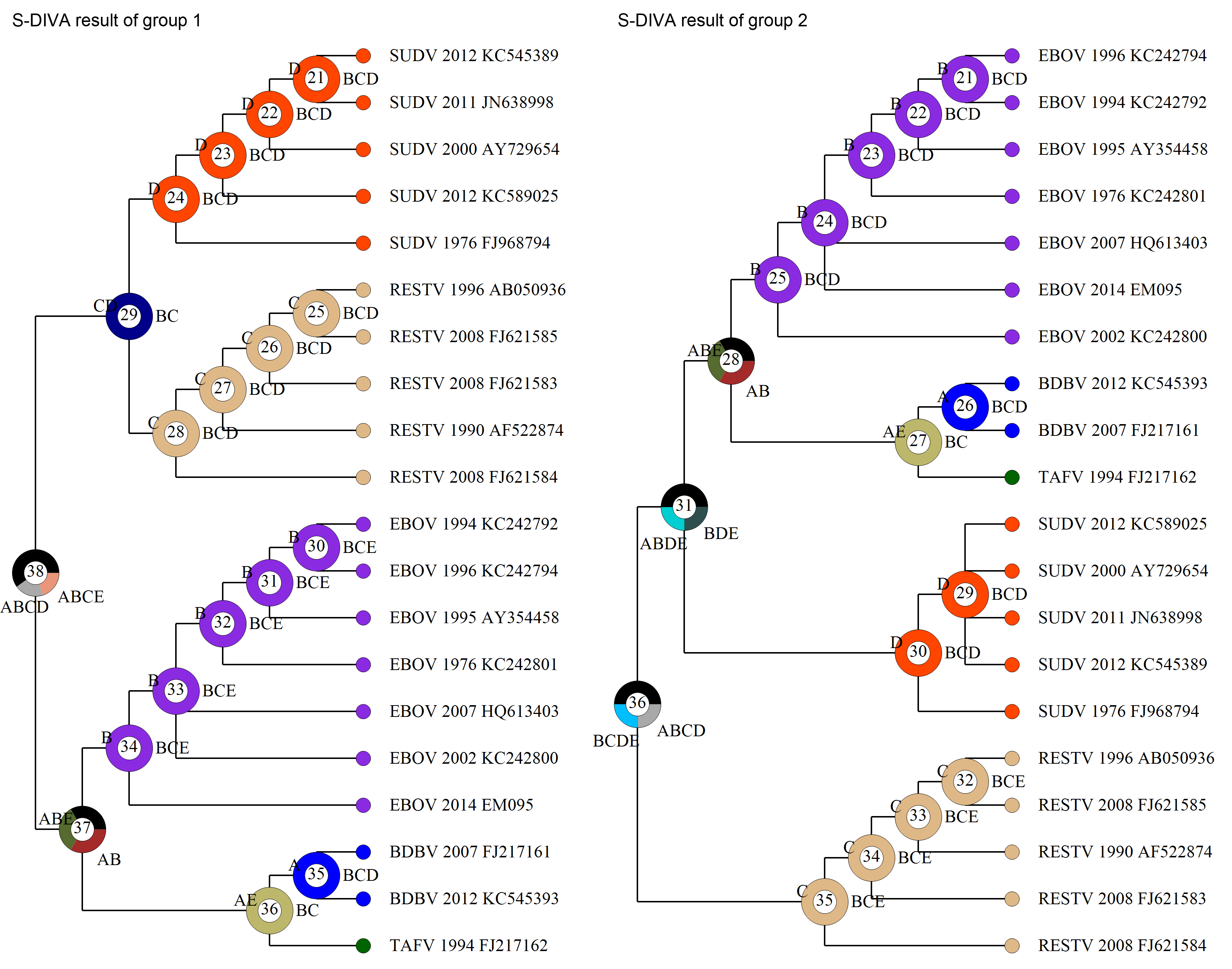
Open [File > Load States (Distributions)], navigate to Trees_States/States.csv and select it. Users can choose the ancestral state reconstruction method based on the data and/or empirical (biological, geographic) considerations. Here we use the S-DIVA method as an example. Open [Reconstruction> On Trees> Statistical Dispersal-Vicariance Analysis (S-DIVA)]. Keep everything as default and click OK. Save the result and graphic in the “Tree  View” window. Users could then do the same steps for group2. The following figures show the contrasting S-DIVA results of group1 and group2. Note that the ancestral states of deeper nodes of the two groups are different.

NOTE: Users can also use Open [File> Load Consensus Tree> Compute Condensed Tree] to compute a binary consensus tree with relative frequencies of clades of trees. Note that the consensus tree generated using RASP does NOT have meaningful branch lengths.

References

Gire, S. K., Goba, A., Andersen, K. G., et al. (2014). Genomic surveillance elucidates Ebola virus origin and transmission during the 2014 outbreak. Science, 345(6202), 1369-1372

Kendall, M. & Colijn, C. (2016). Mapping Phylogenetic Trees to Reveal Distinct Patterns of Evolution. Mol Biol Evol, 33(10), 2735-2743